Optimization passes

CFG Cleanup Pass

GCC jump optimization pass was implemented using simplistic RTL instruction chain analysis and it disturbed control flow graph completely during optimizing.

Since this pass needs to be run many times during compilation and the implementation was somewhat rotten, we have decided to re-implement it completely. In fact the decision predates the project itself and was the first step done in the direction of pushing CFG into compiler. In the first attempt to re implement the pass we failed miserably hitting all sorts of limitations of the control flow graph manipulation code giving us the main motivation for goals of our project.

With important effort spent on the CFG manipulation infrastructure we have succeeded to re-implement all features of old jump optimizer in stronger and faster way. We perform transformations described bellow in the loop until the code stabilizes (ie. no transformation matches after searching the whole flow graph).

Edge Forwarding

The edges whose destination is a ``forwarder block'', where the forwarder block is an empty block or block containing only the unconditional jump instruction, are forwarded to the destination of successor edge of the block.

We have implemented new function to redirect edges in the flow graph and update underlying RTL instruction, that also attempts to simplify branch instruction in the source basic block. When all edges of the computed jump or conditional jump are forwarded to the same destination, the jump instruction is replaced by unconditional jump or removed entirely.

This function is now used in many other places in compiler and this single transformation supersets number of special subcases handled by old jump optimizer code, such as computed jump or table-jump removal.

Jump Threading

Jump threading is an optimization similar to edge forwarding but taking important special case of conditional jump targeting conditional jump with condition whose value can be determined from the condition of first jump. For instance in following code:

$\begin{algorithmic} \IF{$a<0$} \STATE{code not clobbering $a$} \ENDIF \IF{$a>=0$} \STATE{code} \ENDIF \end{algorithmic}$

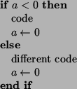
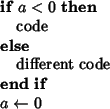
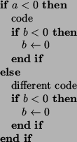
Jump threading adds missing else.

We have implemented jump threading by running CSE over the two basic blocks as if they were a single block. When CSE is able to determine constantness of resulting block we attempt to prove that second basic block has no side effect and forward the edge on success.

Cross Jumping

Cross jumping, also known as tail merging, is a optimization eliminating duplicates in the code. It is identifying sequences of identical code at the end of basic blocks targeting same destination and unifying it. In the simple form it can be used to transform:

$\begin{algorithmic} \IF{$a<0$} \STATE{code} \STATE{$a\leftarrow 0$} \ELSE \STATE{different code} \STATE{$a\leftarrow 0$} \ENDIF \end{algorithmic}$
into:
$\begin{algorithmic} \IF{$a<0$} \STATE{code} \ELSE \STATE{different code} \ENDIF \STATE{$a\leftarrow 0$} \end{algorithmic}$

We implemented generalized form that also identifies control flow transfer instructions that have equivalent effect. This allows, for instance, to transform:

$\begin{algorithmic} \IF{$a<0$} \STATE{code} \IF{$b<0$} \STATE{$b\leftarrow 0$} \... ...fferent code} \IF{$b<0$} \STATE{$b\leftarrow 0$} \ENDIF \ENDIF \end{algorithmic}$
into:
$\begin{algorithmic} \IF{$a<0$} \STATE{code} \ELSE \STATE{different code} \ENDIF \IF{$b<0$} \STATE{$b\leftarrow 0$} \ENDIF \end{algorithmic}$

Such commonalities are surprisingly frequent in the real world code, as they are easily created by function inlining. Also our tracer optimizer increases greatly the amount of cross jumping opportunities. The overall code reduction caused by this optimization is about $10\%$ .

Unreachable Code Removal

We perform simple depth first search through the graph marking all nodes reachable from entry block and removing all unmarked basic blocks.

Unnecessary Code Labels Removal

Code labels that are no longer reached by branch edges are either removed, or converted into DELETED_LABEL notes in case they are still referenced from data segment.

Conditional Jump around Jump Simplification

This transformation simplifies:

$\begin{algorithmic} \IF{$a<0$} \STATE{{\bf goto} skip} \ENDIF \STATE{{\bf goto} branch} \STATE{skip:} \end{algorithmic}$

Into:
$\begin{algorithmic} \IF{$a>=0$} \STATE{{\bf goto} branch} \ENDIF \end{algorithmic}$

Basic Block Merging

In case basic block has a single exit edge that targets other basic block with a single entry edge the basic blocks can be merged. We perform code reordering when needed.

Liveness, CFG and Profile Maintenance

Most importantly our new implementation is transparent to both liveness information and profile. It allows us to run the pass more often producing better code. Also our pass is faster than old implementation, since it does not have to examine RTL chain in detail and can recognize the optimization opportunities on the shape of control flow graph easily.

Loop Optimizer Rewrite

We were unable to adapt the old loop optimizer in GCC to new CFG representation. The reasons were:

It is quite big (14939 lines) and complicated piece of code.
It mostly ignores basic block structure in unrolling part, thus making it very hard to maintain the information.
Its design is not very good; to locate loops, it uses information passed from frontend (notes emitted into insn stream). During former optimization passes, this information often gets mangled, thus preventing the loop optimizer from optimizing the loop.

We have decided to rewrite the loop optimizer from scratch. To keep the functionality, we are slowly replacing it by parts. Till now we have already replaced loop unrolling part and used the created infrastructure to extend it by other natural loop transformations (loop peeling and unswitching).

Loop Data Structure Changes

The old loop optimizer kept information about the loops in a rooted forest (nodes corresponding to loops, edges to subloop/ superloop relation). Basic blocks belonging to a loop were recorded in a bitmap indexed by basic block numbers. This structure was not flexible enough for our purposes - basic block numbers sequentially number basic blocks along insn chain and therefore may change during CFG transformations (a bit unpleasant design choice, making it hard to index anything by them; we are working on changing this). It also was not very efficient for some common operations (for example finding body of a loop required scanning every basic block in the function, finding innermost loop the basic block belonged to was done by testing membership in all the loops).

We decided to change the loop data structure. In our design we came out from the following assumptions:

The loop tree is usually shallow - you will hardly find practical example of program with nested loops.
Loops are not created or destroyed too often.
On the other hand, we relatively frequently change a set of basic blocks that belong to loops.

We have divided the information about loops into parts; one of them is stored in CFG, the other one remains in the loop tree. In the loop tree we store informations describing the loop (pointer to its header and latch, its size), while in CFG we have for each basic block a pointer to the innermost loop it belongs to. Furthermore, we have added a dummy loop containing whole function as a root of the loop tree (making some functions a bit simpler) and for each node of the tree an array of pointers to all its superloops.

With this structure, we are able to provide following operations:

CFG manipulation in .
Queries for membership in loop, innermost containing loop and subloop/ superloop relationship in .
Loop structure changes in $O(\hbox{tree depth})$ .

It is still not straightforward to find a body of the loop; we support this fundamental operation by exploiting natural loop properties (for definition of a natural loop see following section). From the definition it follows that we can enumerate the loop by a simple DFS from the latch backwards along the edges, stopping on the loop header; this is linear in loop size and fast enough for our purposes.

Compared to previous implementation, we only lack possibility of having loops with more than one latch. This is not a problem, as we are always able to eliminate them (as explained in the following section).

Natural Loop Discovery Changes

Natural loop is a maximal (in inclusion) set of basic blocks such that it contains a special one (header) that dominates all of them and is backreachable from them. Predecessors of header inside loop are called latches. If there is a single predecessor of header outside the loop, we call it a preheader.

Natural loop discovery code (based on ...) was provided by Michael Hayes (but it was not used in loop optimizer yet); we only had to adapt it for a new loop infrastructure. In following paragraphs we address some issues concerning the change.

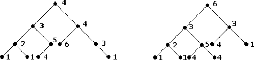
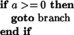
As mentioned earlier, our data structure does not support loops with more than one latch basic block. This is not a great problem, as such loops are somewhat nonstandard and we would have to bring them into a canonical shape anyway. Loop with more latches can occur from the following reasons:

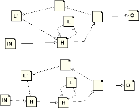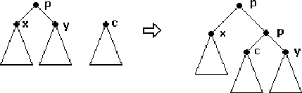
Presence of the inner loop with the shared header. The correct way to eliminate this case is to create a new empty header for the outer loop. $\resizebox{!}{50mm}{\includegraphics{inner_loop.ps}}$
Several branches inside loop ending in the header; we eliminate this by creating a new empty latch. $\resizebox{!}{50mm}{\includegraphics{two_branches.ps}}$

It is relatively hard to distinguish these cases (but they are not too common anyway, so it is not too important). If we have profile information, we can differ between them; while in the latter case frequencies of the latch edges are similar, in the former case latch edge of inner loop tends to be much more frequent. Otherwise we simply use the second way.

In addition, we have also provided some functions to bring loops into even more canonical shape (creating preheaders; forcing preheaders/latches to have only a single outgoing edge to the loop header) in that it is much easier to keep the loop structure up to date during transformations like loop copying etc.

Loop Optimizer

We started our work on new loop optimizer by replacing the part responsible for most structural changes - the unroller. We have postponed work on other optimizations (induction variable elimination, strength reduction) until we have mid-level RTL and SSA form that should make the work much easier.

We have implemented basic functions for CFG manipulation able to update loop structure (and also to keep dominator tree up-to-date, which is important for some of our optimizations).

Using them, we have created several useful functions for loop structure manipulation (copying of loop body to the edge coming into its header - operation common for both loop unrolling and peeling, removing the branch of if condition inside loop - for unswitching and clever loop unrolling, loopification of a part of the CFG, creating a canonical description of simple (in sense that we are able to determine number of their iterations) loops).

We are able to keep profiling information consistent in most of the times (the only place where we have problem is removing branches; it is hard to recalculate frequencies precisely afterwards, so we only use some approximation).

Loop Unrolling

By loop unrolling we mean copying the loop body several times. The result is that in a loop that iterates often enough we create longer run of instructions that are executed sequentially (without jumps). Such code is often executed faster.

while (1) { puts("Header"); if (should_end ()) break; puts("Latch"); } while (1) { puts("Header"); if (should_end ()) break; puts("Latch"); puts("Header"); if (should_end ()) break; puts("Latch"); puts("Header"); if (should_end ()) break; puts("Latch"); }
$\resizebox{!}{60mm}{\includegraphics{unroll_simple.ps}}$

With the described machinery, unrolling is quite easy - it suffices to copy loop body on the edge from latch to header.

This stupid loop unrolling is not always a win; it makes code to grow, which may cause problems with caches, making the program to run slower. To avoid this, we only unroll small loops. With profile informations, we only unroll loops that are expected to iterate often enough and also disable the optimization on places that do not execute often enough.

We have also written some more clever variants of the basic loop unrolling scheme:

for (i = 0; i < 10; i++)
 printf ("%d\n", i);

$\downarrow$

i = 0;
while (1)
 {
  printf ("%d\n", i++);
  if (i>=10)
   break;
  printf ("%d\n", i++);
  printf ("%d\n", i++);
 }




for (i = 0; i < k; i++)
 printf ("%d\n", i);

$\downarrow$

i = 0;
m = (k - i) % 3;
if (!m--)
 goto beg;
if (i>=k)
 goto end;
printf ("%d\n", i++);
if (!m--)
 goto beg;
printf ("%d\n", i++);
beg:
while (i < k)
 {
  printf ("%d\n", i++);
  printf ("%d\n", i++);
  printf ("%d\n", i++);
 }
end:;

$\resizebox{105mm}{!}{\includegraphics{unroll_clever.ps}}$

Unrolling Loop With Known Number Of Iterations

If we are able to determine the number of loop iterations exactly, we can either peel the loop completely (removing the loop) if it is sufficiently small, or at least determine precisely the exit that will be taken out of the loop (by counting the number of iterations modulo the number of unrollings). We can then remove exit edges that we know that are not used.

Unrolling Loop With Number Of Iterations Known At Runtime

Often it happens that we are not able to count number of iterations in time of compilation, but we are able to count it in runtime. Then we can add code to ensure that number of iterations is divisible by number of unrollings (by peeling loop several times and adding conditions to check that correct number of iterations is remaining, then unroll the loop and remove exit tests from all but one copy of body.

This is not the whole story, as in this case we have to count with some degenerated instances. The easy one is that the loop may not roll at all; this we can check rather easily. More difficulties arise from the fact that we also have to check for overflows. Fortunately, if the number of times we unroll the loop is a power of , this will not cause the problems (as overflows only occur in case the the final check is for equality and range of integer types is power of , therefore modulo number of unrollings the result is the same).

In both of these cases we benefit not only from greater sequentiality of code, but also from removing the unnecessary checks and better possibilities for further optimizations.

Loop Peeling

while (1)
 {
  puts("Header");
  if (should_end ())
   break;
  puts("Latch");
 }

$\rightarrow$

puts("Header");
if (should_end ())
 break;
puts("Latch");
puts("Header");
if (should_end ())
 break;
puts("Latch");
while (1)
 {
  puts("Header");
  if (should_end ())
   break;
  puts("Latch");
 }

$\resizebox{60mm}{!}{\includegraphics{peel.ps}}$

Peeling is similar to unrolling, but instead of copying loop to latch edge, we copy it to preheader edge, thus decreasing the number of loop iterations. Peeling is used if number of loop unrollings is small; the resulting code is again more sequential.

Loop Unswitching

i=10;
while (1)
 {
  if (flag)
   puts("True");
  else
   {
    puts("False");
    if (!i--)
     break;
   }



 i=10;
 if (flag)
  while (1)
   puts("True");
 else
  while (1)
   {
    puts("False");
    if (!i--)
     break;
   }
 }

$\resizebox{!}{60mm}{\includegraphics{unswitch.ps}}$

Loop unswitching is used in case when some condition tested inside loop is constant inside it. Then we can move the condition out of the loop and create the copy of the loop. Then in the original loop we can expect the condition to be true (and remove the corresponding branch) and in the copy to be false (and again remove the branch).

We must be a bit careful here, as if we had several opportunities for unswitching inside a single loop, the code size could grow exponentially in their number. Therefore, we must have some threshold over that we will not go.

Other interesting case is when we test for the same condition several times. We can then use our knowledge of which branch we are in to just eliminate the incorrect path; the only small problem associated with this is that we could create unreachable blocks, or even cancel the loop. Both of these cases are hard to handle, so we just revert to former case (it does not occur too often, and the following optimization passes will get rid of that much apparently unreachable code anyway).

ET-Trees

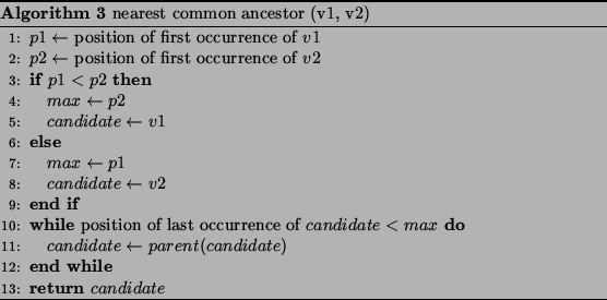
We used ET-trees for maintaining dominance information in loop optimizer. ET-tree is a data structure for representing trees. It offers logarithmic time for standard tree operations (insert, remove, link, cut) and poly-logarithmic time for finding common ancestor of two nodes.

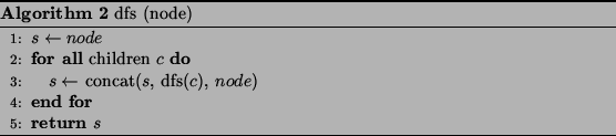
The tree is represented by a sequence of symbols obtained by calling algorithm on root node.

$\begin{algorithm} % latex2html id marker 1404\caption{dfs (node)}\begin{algori... ...$c$), $node$)} \ENDFOR \STATE{{\bf return} $s$} \end{algorithmic}\end{algorithm}$

Such sequences are called Eulerian Tours, hence the name of the structure. For example, for tree on figure , the corresponding ET-sequence is 1,2,1,3,4,5,4,6,4,3,1.

**Figure:** A tree with ET-sequence 1,2,1,3,4,5,4,6,4,3,1
$\scalebox{1.0}{ \includegraphics{et-tree1.ps}}$

Because it's inefficient to maintain these sequences as strings, slightly different approach is used -- the sequence itself is represented by a binary tree, where the represented sequence is obtained by reading the values of the nodes from left to right.

For example, two possible encodings of the above sequence are shown in figure .

**Figure:** Two possible encodings of the above sequence.
$\scalebox{0.9}{ \includegraphics{et-tree2.ps}}$

In our implementation, we have chosen splay-trees as the sequence representation, with some modifications:

All occurrences of the same node are linked from left to right, this allows faster implementation of remove.
Because node values can be of any type, a hashtable is used to convert node values to appropriate internal representation.

There are two data types for representing nodes -- et_forest_occurrence and et_forest_node. et_forest_occurrence represents the occurrences of the nodes in tree (therefore, these nodes form the splay-tree). It contains informations for the splay-tree (parent node, left son, right son), pointer to the next occurrence of the same node, and number of nodes in left and right subtree (this is used for comparison whether an occurrence is before another one, or not). et_forest_node represents each node. It contains pointers to the first and last occurrences of the node and the node value. The et_forest_t is then simply a hashtable converting node value to appropriate et_forest_node.

Implementation of of tree operations

Insertion of new node is trivial -- we simply create a node with one occurrence.
Insertion of an edge -- we splay first occurrences of both nodes, create new occurrence of parent node and link them together as shown in figure .

Figure: Insertion of edge (p,c).

$\scalebox{1.0}{ \includegraphics{et-tree3.ps}}$
Removal of a node -- We simply remove edges to child nodes and possibly the edge to parent node and then dispose the node with single occurrence.
Removal of an edge -- Because we know that the occurrences before the first occurrence of child node and after the last occurrence of child node belongs to parent node, we cut the sequence using two splays and one join, removing one occurrence of parent node, as shown in figure .

Figure: Deletion of edge (p,c).

$\scalebox{1.0}{ \includegraphics{et-tree4.ps}}$
Nearest common ancestor of two nodes is calculated by algorithm .
$\begin{algorithm} % latex2html id marker 1455\caption{nearest common ancestor ... ...e)$} \ENDWHILE \STATE{{\bf return} $candidate$} \end{algorithmic}\end{algorithm}$
Splay trees are well known and therefore not covered here.

**Figure:** Insertion of edge (p,c).
$\scalebox{1.0}{ \includegraphics{et-tree3.ps}}$

**Figure:** Deletion of edge (p,c).
$\scalebox{1.0}{ \includegraphics{et-tree4.ps}}$

Register Coalescing Pass

We found another irritating defect of GCC register allocation pass -- the fact that it is not able to eliminate redundant register to register copies. The copies are commonly created as a result of global common subexpression elimination (GCSE) pass and resulting code is often slower than when GCSE is disabled. In our efforts we have fixed some defects of GCSE resulting in more changes to be done making this problem serious. This was the main motivation to implement simple register coalescing pass.

The pass first scans function and builds conflict graph of pseudo registers (vertexes of graph are registers and two registers are connected by edge when they are live together, so they cannot reside both in a single register). Later the program is rescanned and each register-to-register copy operation is considered. When there is no edge between both operands of the copy, the registers are marked for coalescing and conflict graph is updated. Finally the instruction chain is updated to represent the coalesced form.

We have found this pass to be relatively effective (eliminating all negative effects of GCSE), however we are not sure whether it will be merged to mainline GCC, as new register allocation branch already contains register allocation able to handle the situation in question. We are considering extending the pass to replace current GCC regmove pass, that is doing essentially the same, but its purpose is to convert RTL chain into form representable in 2 address instruction set (if target architecture has one), when the destination of operation is equivalent to its source.

First we need to discuss with register allocation developers what level this transformation should be done on. Also it is possible that the new register allocation will not be merged into mainline tree until the next release, in that case we will attempt to merge our pass as a temporary solution.

Webizer

Modern register allocation algorithms are usually not based on pseudo registers, like the GCC one, since pseudo registers representing variables may be reused for no real purpose. For instance many programmers are using i in the single function as index counter in many different loops. It is stupid to constraint register allocator to allocate single hardware register for all occurrences of variable i.

Solution to this problem is to split each pseudo register into one or more webs. The name web comes from DU data-flow representation. In this form, each definition of register has an attached linked list pointing to all instructions possibly using the value (Definition Use chains). The webs can be constructed by unifying all definitions having the same uses (as when instruction uses value from multiple possible definitions, all definitions must come to the same register).

We have implemented simple pass that constructs DU chains, computes webs and when single pseudo has attached multiple webs, it creates new pseudo register, so at the end there is correspondence between pseudo registers and webs.

This allows register allocation to be stronger without additional modifications. In addition this makes some other optimization passes stronger. For instance the following piece of code
$\begin{algorithmic} \STATE {$a\leftarrow a+1$} \STATE {$b[a]\leftarrow 1$} \STAT... ...w a+1$} \STATE {$b[a]\leftarrow 1$} \STATE {$a\leftarrow a+1$} \end{algorithmic}$

after webizing looks like:

$\begin{algorithmic} \STATE {$a\leftarrow a+1$} \STATE {$b[a]\leftarrow 1$} \STAT... ...1$} \STATE {$b[a_3]\leftarrow 1$} \STATE {$a\leftarrow a_3+1$} \end{algorithmic}$

and GCC Common Subexpression Elimination pass converts it into:

$\begin{algorithmic} \STATE {$a\leftarrow a+1$} \STATE {$b[a]\leftarrow 1$} \STAT... ...w 1$} \STATE {$b[a+2]\leftarrow 1$} \STATE {$a\leftarrow a+3$} \end{algorithmic}$

when offsetted addressing is available. We run Webizer twice -- once in early compilation stages and once after tracing and loop unrolling, so we do not need to implement special purpose pass to split induction variables.

Software Trace Cache

Theory

We use a greedy algorithm similar to Software Trace Cache [7] for basic block reordering. It reorders basic blocks to minimize the number of branches and instruction cache misses and does also a limited amount of code duplication during the process to avoid jumps. The effect is the increase of code sequentiality and thus also the increase of the speed of code execution.

The algorithm is based on profile information. It means that the results depend on the representativity of the training inputs. Thus the code can be worse for some input sets. If you have not profiled the program the algorithm uses the probabilities of branches estimated by a set of heuristics instead of profile information.

We minimize the number of (executed) branches by constructing the most popular sequences of basic blocks (the traces). To do that we are reordering the most probable successor after its predecessor. If the most probable successor has been already laid out we duplicate it to avoid jump if we are not duplicating a large chunk of code. A trivial example of duplication is copying the return instruction instead of jumping to it.

Implementation

The implementation does only intra-procedural optimizations since inter-procedural optimizations are out of reach of current GCC.

The algorithm constructs traces in several rounds. The construction of traces starts from the selected starting basic blocks (seeds). The seeds for the first round are the entry points of the function. When there are at least two seeds the seed with the highest execution frequency is selected first (this places the most frequent traces near each other to avoid instruction cache misses). Then the algorithm constructs a trace from the seed by following the most probable successor. Finally it connects the traces.

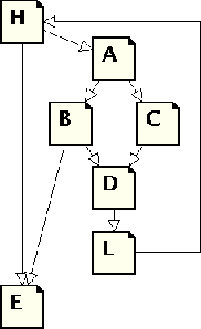
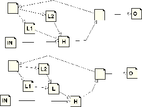
As we mentioned before the most frequently executed seed is selected. But there are some exceptions: The seeds whose predecessors already are in any trace or the predecessor edge is a DFS back edge are selected before any other seeds. This heuristics tries to create longer traces than the algorithm would create without this heuristics. In figure , the blocks H, A, B and E are already in a trace, the seeds are C and D. The seed C will be selected first because all its predecessors are already in some trace, even if the execution frequency of D is higher.

**Figure:** Selecting seed `C' before `D'
$\scalebox{.5}{ \includegraphics{stc_seed.ps}}$

Given a basic block, the algorithm follows the most probable successor from the set of all unvisited (ie. not in any trace) successors and visited successors that can be copied. The decision whether the visited block can be copied is done by simulation of the trace building and counting the number of bytes that would be copied. The block can be copied only if the size that would be copied is lower than a threshold. The threshold depends on the size of the jump instruction and on the frequency of the block.

While constructing the trace the algorithm uses two parameters: Branch Threshold and Exec Threshold. These parameters are used while scanning the successors of the given block. If an edge to a successor of the actual basic block is lower than Branch Threshold or the frequency of the successor is lower than Exec Threshold the successor will be the seed in one of the next rounds. Each round has the Branch Threshold and Exec Threshold less restrictive than the previous one. The last round has to have these parameters set to zero so that the last round could "pick up" remaining blocks. The successors that has not been selected as a continuation of the trace and has not been "sent to" next rounds will be added to seeds of current round and the secondary traces will start in them.

There are several cases of the selected successor's state (the action for the first matching state will be done):

The duplicate of the successor is in this trace. We have found the loop in original flow graph. The algorithm terminates the construction of the trace.
The successor has been visited in this trace. We have found the loop that is rotated if it is profitable. The construction of the trace is terminated.
The successor has been visited (not in this trace). It is duplicated and the duplicate is added to the end of the trace.
Otherwise. It is added to the end of the trace.

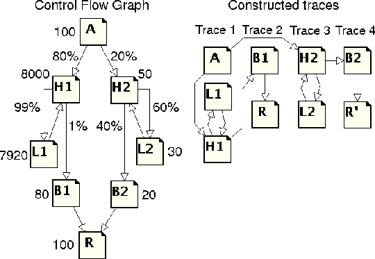
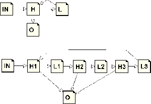
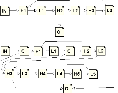
Figure shows an example of the flow graph. We use an Exec Threshold of 50 and Branch Th. of 30% in the first round. Given a seed A we follow the edge to H1, and H2 is sent to next round because of Branch Th. We continue to L1 from H1, B1 is sent to next round. The best (and the only) successor from L1 is H1. We have found a loop that has enough iterations so we rotate it and terminate the trace. There are no more seeds in this round so the next round starts. We use Branch Th. of 0% and Exec Th. of 0 so this is the last round. The seed B1 has higher exec count than H2 so the next trace starts in B1. We follow the edge to R and terminate the trace because the block R is the exit block of the function (in GCC representation, there is an edge from R to EXIT_BLOCK). Next trace starts in H2 and continues to L2, B2 will be a seed for secondary trace. In L2, we find a loop that does not have enough iterations so we just terminate the trace. The last trace starts in B2. The successor R is already in some trace so we check whether we can duplicate it and realize that we can. So we duplicate it. Since it is the exit block of function, we terminate the trace. There are no more unvisited blocks so the trace building is done.

**Figure:** Trace building
$\scalebox{.5}{ \includegraphics{stc_traces.ps}}$

Finally we connect the traces. We start with the first trace (that contains the entry block of function). Given a chunk of connected traces we prolong it. If there is an edge from the last block of the chunk to the first block of some trace that trace will be added to the end of the chunk. If there is no such trace the next unconnected trace is added to the chunk.

For the graph in figure , the traces happen to be connected in the same order as they were found.

Tracer

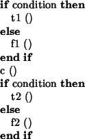
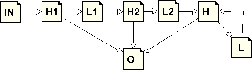
Tracer [2] performs the tail duplication which is needed for superblock formation. Usually it is used for scheduling but we have not tested it because GCC does not have general Superblock Scheduler (GCC has it only for IA-64) but we plan to generalize it in the future. We do not suppose that the scheduling will be profitable for Athlon (where we tested everything) because Athlon itself does the scheduling. On Athlon, we use Tracer to improve the effect of other optimizations. We do not need to worry about the code growth too much because Cross-jumping removes the unneeded tail duplicates when optimizations are not performed. The simple example how tracer helps other optimizations is the following code. Tracer makes possible for CSE to remove the second condition.

Example: Code where Tracer helps other optimizations.
$\begin{algorithmic} \IF{condition} \STATE{t1 ()} \ELSE \STATE{f1 ()} \ENDIF \STATE{c ()} \IF{condition} \STATE{t2 ()} \ELSE \STATE{f2 ()} \ENDIF \end{algorithmic}$

The start trace finding from the basic block that is not in any trace yet and has the highest execution frequency. The Fibonacci heap is used for fast finding of such a block. The trace is then grown backwards and forwards using mutual most likely heuristic. The heuristic requires that for block A that is followed by block B in the trace, A must be B's most likely predecessor and B must be A's most likely successor. While the trace is growing backwards the backward growing can also stop if the probability of the most likely predecessor is lower than MIN_BRANCH_RATIO and while the trace is growing forwards the growing can also stop if the probability of the most likely successor is lower than MIN_BRANCH_PROBABILITY.

When we have a trace we perform tail duplication. We visit the blocks on the trace in trace order, starting with the second block. If a block has more than one predecessor the block is duplicated (with all outgoing edges) and the edge from previous block of the trace is redirected to the duplicate. This is repeated until every basic block on the trace is visited.

The trace finding and tail duplication is repeated until we cover the ratio of DYNAMIC_COVERAGE of the number of dynamic instructions (number of executed instructions in the function). The process also stops when the number of instructions exceeds MAXIMAL_CODE_GROWTH multiplied by the original number of instructions because we have to keep code growth and compiler resources under control although the unneeded duplicates will be eliminated later in Cross-jumping. The remaining basic blocks are the traces of one basic block.

Finally the traces are connected into one instruction stream. When there is an edge from the last basic block of one trace to the beginning of another these traces will be connected. Remaining chunks are connected in the order of appearance. We do not need to worry how well the traces will be connected because Basic Block Reordering will order the blocks so that the code will be (almost) as fast as possible.

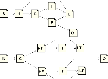
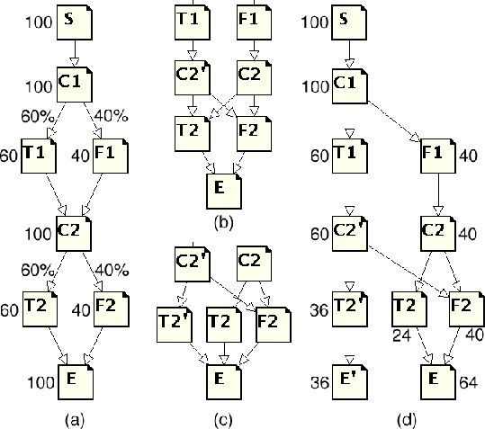
Figure .a shows the original flow graph for an example code on page . We start finding the trace in basic block S since it has the highest execution frequency. The trace is grown forwards by basic blocks C1, T1, C2, T2 and E. While visiting the blocks on the trace in trace order we duplicate block C2 because it has two predecessors. Basic block T2 has two predecessors now because of duplication of C2 (see figure .b) so we duplicate it too (see figure .c). Finally we duplicate basic block E too. Figure .d shows the result after tail duplication of the first trace. We start finding next trace in E. The trace grows backwards by basic block F2. It cannot grow by C2 because F2 is not the most likely successor of C2. The basic block E is then duplicated. The finding of next trace starts in basic block F1 and grows forwards by blocks C2, T2 and E. All basic blocks in this trace have one predecessors so no basic blocks are duplicated now. There are no more basic blocks left. The first trace is S, C1, T1, C2', T2', E', the second one is F2, E'' and the last one is F1, C2, T2, E.

**Figure:** (a) The original flow graph for example code on page . (b) A part of flow graph after duplicating C2. (c) A part of flow graph after duplicating T2. (d) The flow graph after tail duplicating the first trace.
$\scalebox{.5}{ \includegraphics{tracer.ps}}$

Code Alignment

The modern CPUs are usually getting instruction decoder stalls when branch targets are near code cache-line boundary. To avoid the problem, the targets of common branches and bodies of loops are recommended to be aligned to start at new cache-line boundary. Also when proceeding a code block that is rarely executed, targeting the branch just before cache-line boundary is wasteful concerning the code cache pollution.

Old GCC contained code to align all loops found in the code, all function bodies and all code following unconditional jumps to specified values according to target machine description. This strategy is however somewhat wasteful. For instance AMD Athlon chip recommends to align to 32byte boundary wasting 16 bytes up to 20% of code at the average.

We have implemented new pass that uses profile to carefully place alignments. We use the following set of conditions:

in case basic block is not reached via fallthru edge check:
- basic block is likely to be executed at least once
- the sum of branch frequencies is very high (1/10th of maximum inside function) or the previous basic block is unlikely executed
If both conditions hold, the basic block is aligned by the same alignment as old code did for instruction following unconditional jump.
in case basic block is reached by both fallthru and branch edge check:
- basic block is in the hot spot of the program
- the sum of frequencies of branch edges is at least 5 times higher than fallthru edge frequency
- basic block is in the very hot spot in the function
If all the conditions are met, the basic block is aligned by loop alignment.

We have found that our code limits code growth to 5% while maintaining approximately the same performance in all benchmarks.

Miscellaneous Changes to Existing Optimizers

We have modified following existing optimizers to use profile feedback:

register referencing: Register referencing pass decides what register class the given pseudo register should be allocated in. This is done by combining preferences of all instructions mentioning the given register. We now weight the preferences by expected frequencies of basic blocks.
register allocation: GCC register allocator simply assigns each pseudo register a priority and then allocates registers to pseudo registers in the priority order giving each pseudo register the first register available in its preferred class and then the first available register in the alternate class if it did not succeed in the preferred class.
We have modified the code to compute pseudo register priority to use frequencies instead of simple loop depth heuristics and have important success with this change speeding up the resulting code by about 0.6%.
final pass: Final pass outputs code alignment recommended for function body by target machine description. We omit the alignment, where allowed, for functions not executed in the training run when profile feedback is available.
register-stack conversion: Register stack conversion pass has property that it always produces code optimal only for one entry path to each basic block. We have modified its traversal to take into account frequencies in order to optimize the most frequent paths.

Double test conversion pass

Double test conversion pass is a pass discovering conditionals in the form of (cond1||cond2) or (cond1&&cond3) and contained in the same superblock and attempts to construct equivalent sequences without branch instruction. In the trivial case a||b this can be done by converting into arithmetics a|b that in i386 instruction set even compiles into equivalently long code in case both variables are present in registers.

The idea can be generalized for example to convert, for instance, a==x||a==y into (a^x)|(a^y). We have implemented special function attempting to convert conditional into expression that is non-NULL when conditional is true, and use it to combine two instructions, algebraically simplify the resulting expressions and test whether resulting sequence is probably cheaper than the former. If so, we do the replacement.

We measured this optimization to improve SPEC2000 performance by about $0.3\%$ . We expect the transformation to be more successful on EPIC architectures, but we have not tried it yet.

Jan Hubicka 2003-05-04